Fast, Interpretable, and Deterministic Time Series Classification with a Bag-Of-Receptive-Fields

When working with time series classification, the most accurate models today are often convolution-based methods such as ROCKET, MiniRocket, Hydra, and InceptionTime, or hybrid models like MR-Hydra. These approaches represent time series in highly complex, non-interpretable feature spaces. Their strengths are clear: they are both accurate and efficient. But they also come with downsides: they are often opaque, making it hard to understand their decisions, and they can be non-deterministic, producing slightly different outputs each time they run.

On the other hand, interpretable models, such as shapelet-based (ST, RDST), interval-based (DR-CIF, RSTSF), and dictionary-based (MR-SEQL, MR-SQM, WEASEL+MUSE), focus on building features that are more interpretable for humans. These methods are reasonably accurate and efficient, and, most importantly, interpretable. However, even here, many remain non-deterministic.

The goal of the Bag-of-Receptive-Fields (BORF) is to design a time series transformation that is accurate, efficient, interpretable, and deterministic, all at once.

From Bag-of-Patterns to Bag-of-Receptive-Fields

One early interpretable approach is the Bag-of-Patterns (BOP) by Baydogan et al. (2013). It works by extracting small “words” from a time series and counting how often they occur.

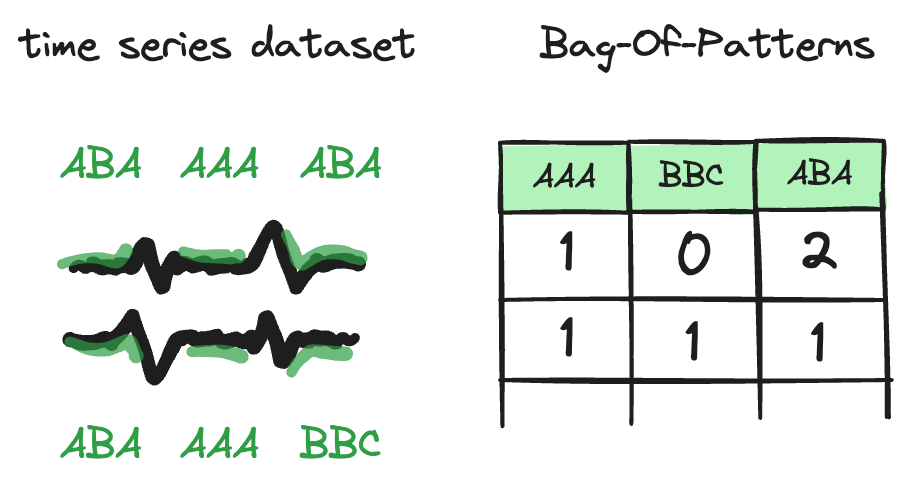
BOP’s advantages are its determinism and interpretability. But it is inefficient, achieves relatively poor accuracy, and was originally limited to univariate series only. Our work improves and extends BOP into the Bag-of-Receptive-Fields (BORF), addressing these limitations.

We try to solve some of these issues with BORF.

BORF

Step 1. - PAA (Naive)

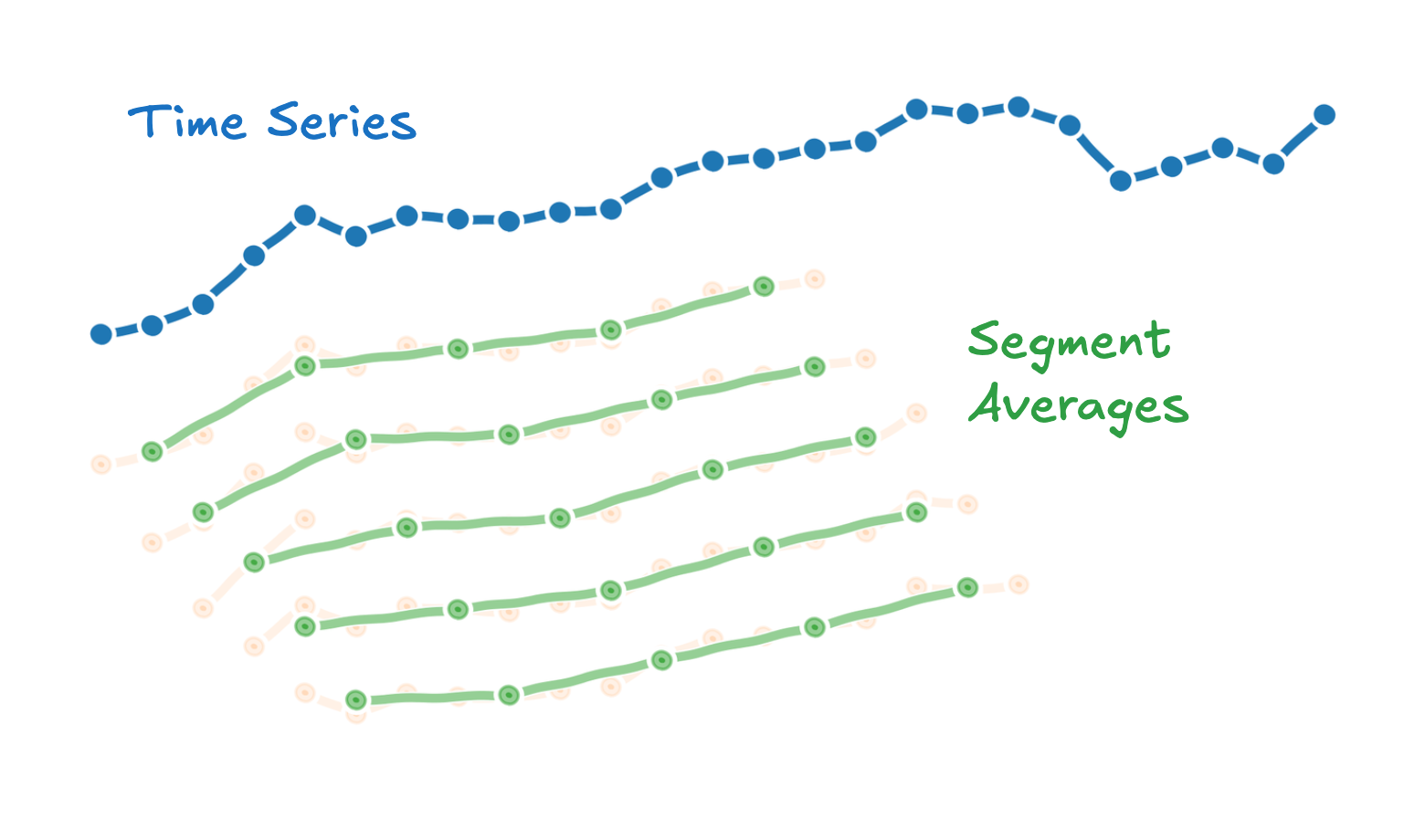
BORF is built on Piecewise Aggregate Approximation (PAA). Given a univariate time series $X$, of length $m$, the naive method, used in BOP, works like this:

Sliding Window

Extract all possible $v$ windows of length $w$ from the time series (we visualize only the first five in the image).

Segmenting

Split each window into $l$ segments of length $q$ (assuming $w$ divisible by $l$).

Averaging

Take the average of each segment.

The problem with this naive approach is its complexity:

This can be quadratic in the length of the time series, i.e., $O(m^2)$, for a sufficiently big $w$.

Step 1. - PAA (Optimized)

The PAA values can be stored in a matrix of shape $v\times l$:

So, if we precompute all possible segment averages, we should be able to collect them by iterating on $v\times l$ entries, instead of $v\times w$ as before. Indeed, the naive computation repeats averages unnecessarily. Instead, we compute each segment average once, using a moving average, $\boldsymbol\mu^{\textit{seg}}$, with a window equal to $l$, and collect them into $M$:

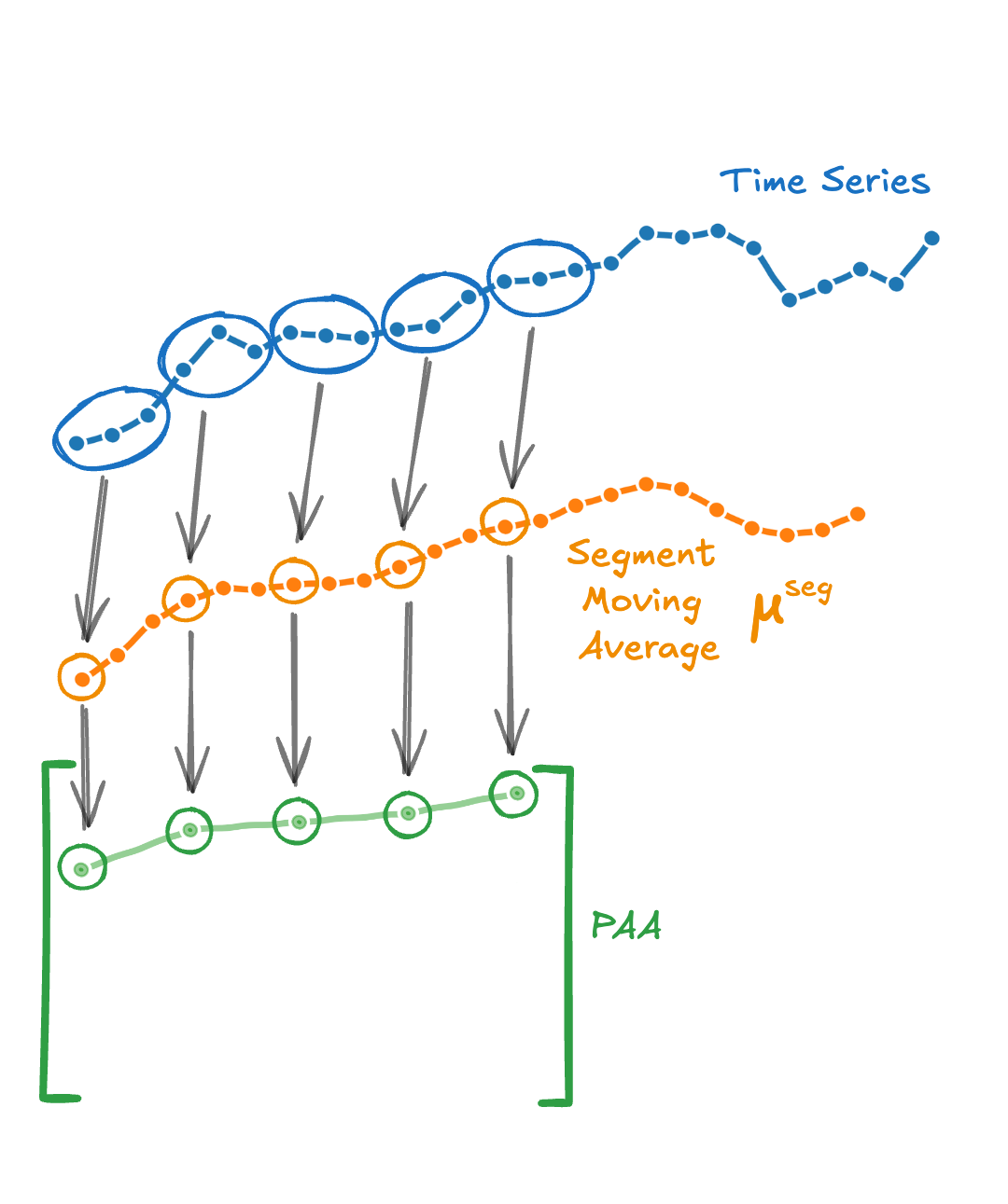
The formula complicates slightly if we borrow dilation ($d$) and stride ($s$) from convolution-based methods to define receptive fields:

In this case the segment can skip observations, and the windows may not be contiguous. A small detail here is that, to compute the moving average with dilation $d$, we partition the time series into $d$ interleaved subsequences, compute a standard length-$q$ moving average on each subsequence and then interleave the results back to the original index order.

This gives an optimized complexity:

In practice, this means that the complexity is independent from the window length, and depends only on the word length. This is very useful as the length of the time series grows.

Step 2. - SAX

Once we have the averages, we normalise each using its window mean and standard deviation (again computed as moving quantities):

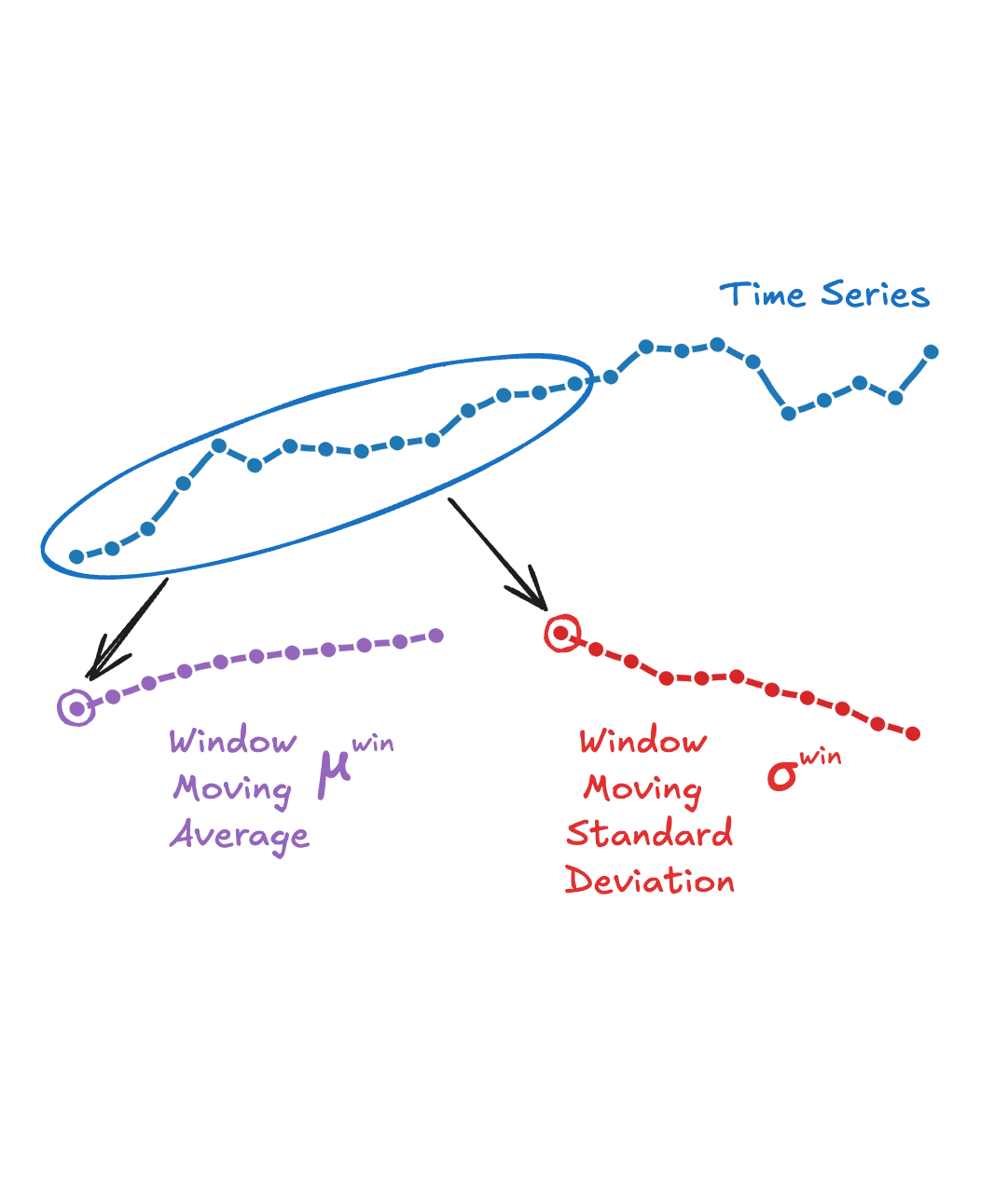
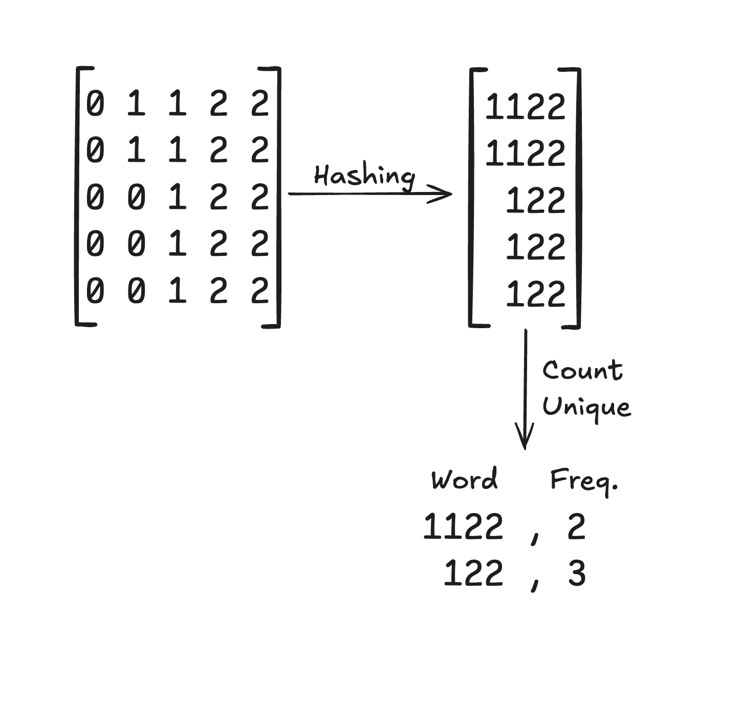
We then bin these values into symbols according to a chosen alphabet size:

Next, we hash the symbol sequences (our “words”) into integers and count their frequency:

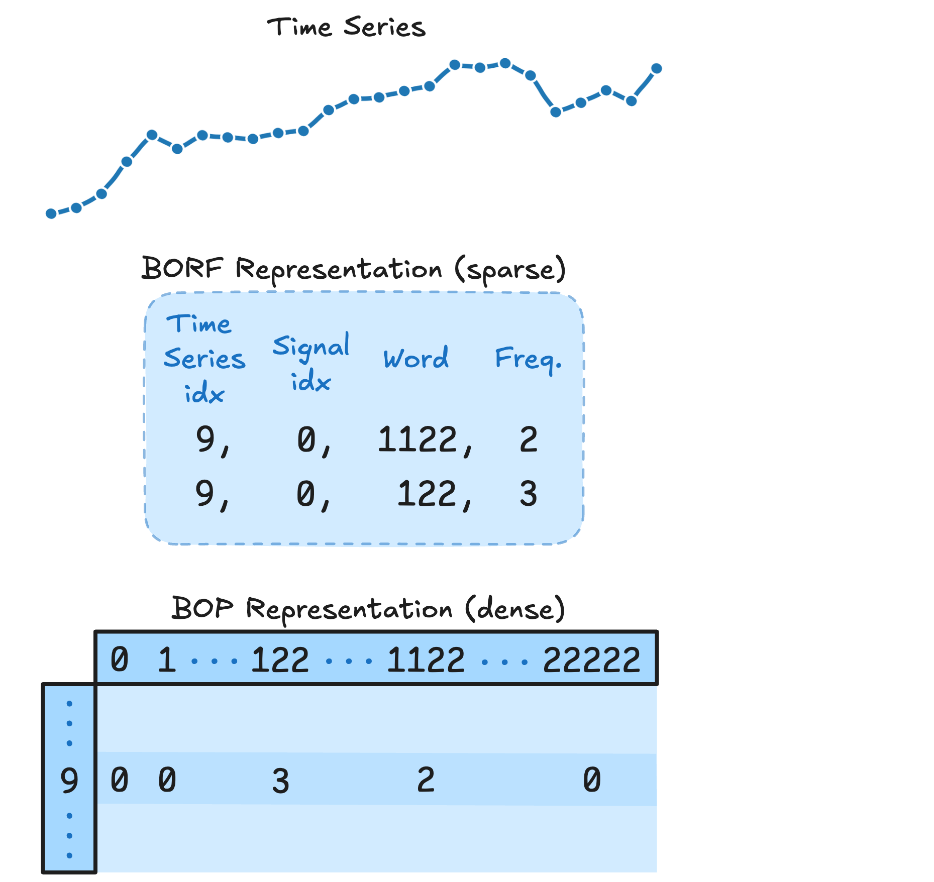
Finally, we record them as a sparse coordinate tensor (COO format), keeping track of which time series and signal each pattern came from:

Multiple Representations

To capture patterns at different scales, we repeat the process using multiple parameter combinations:

• Window lengths: $[2^2, 2^3, \dots]$
• Dilations: $[2^0, 2^1, \dots]$
• Word lengths: $[2, 4, 8]$

We fix the alphabet size to 3, set stride to 1, and flatten + concatenate all features.

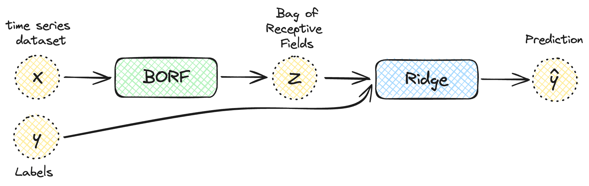
BORF is implemented in the aeon library and can be plugged into any machine learning pipeline.

Performance and Explanation

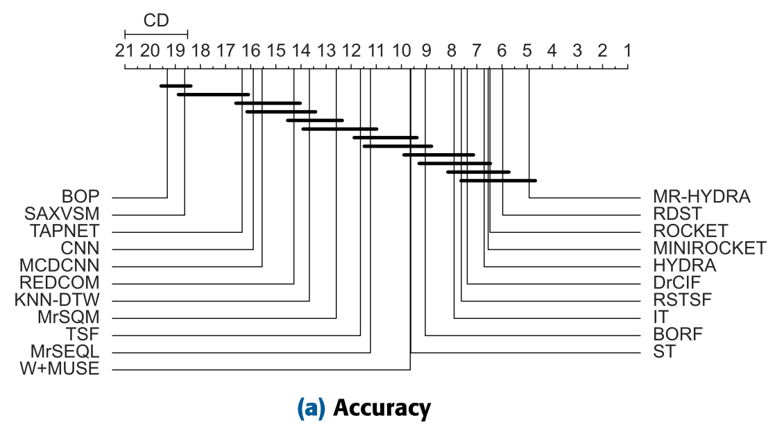
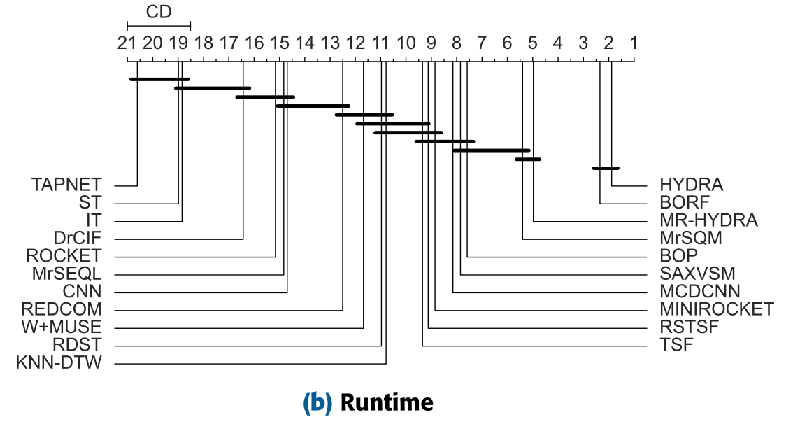
On the UEA and UCR benchmarks, BORF shows strong accuracy while being much faster than many competitors.

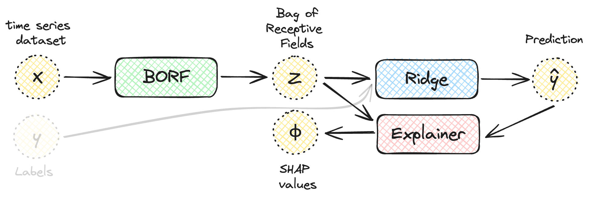
Because BORF produces a tabular representation, we can apply standard explainability methods like SHAP:

On the CBF dataset, we can inspect both local and global explanations:

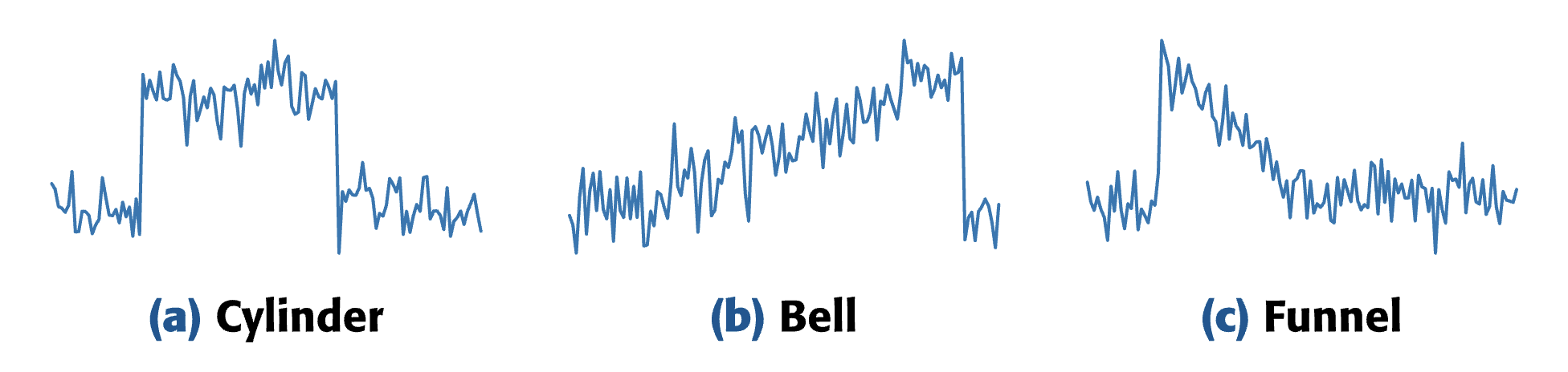
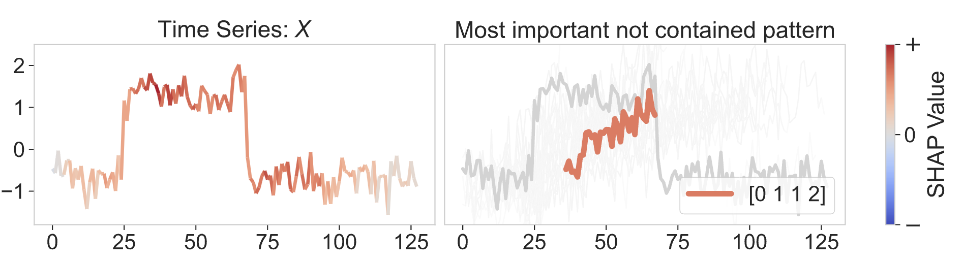
The picture below shows an instance correctly classified as a Cylinder. On the left, we show a saliency map, obtained by mapping the importance of each contained pattern back to the original time series. The most important points seem to be in the center of the time series, with the edges mainly composed of noise.

On the right, we show the most important absent pattern (0,1,1,2 or low-medium-medium-high), a rising one.

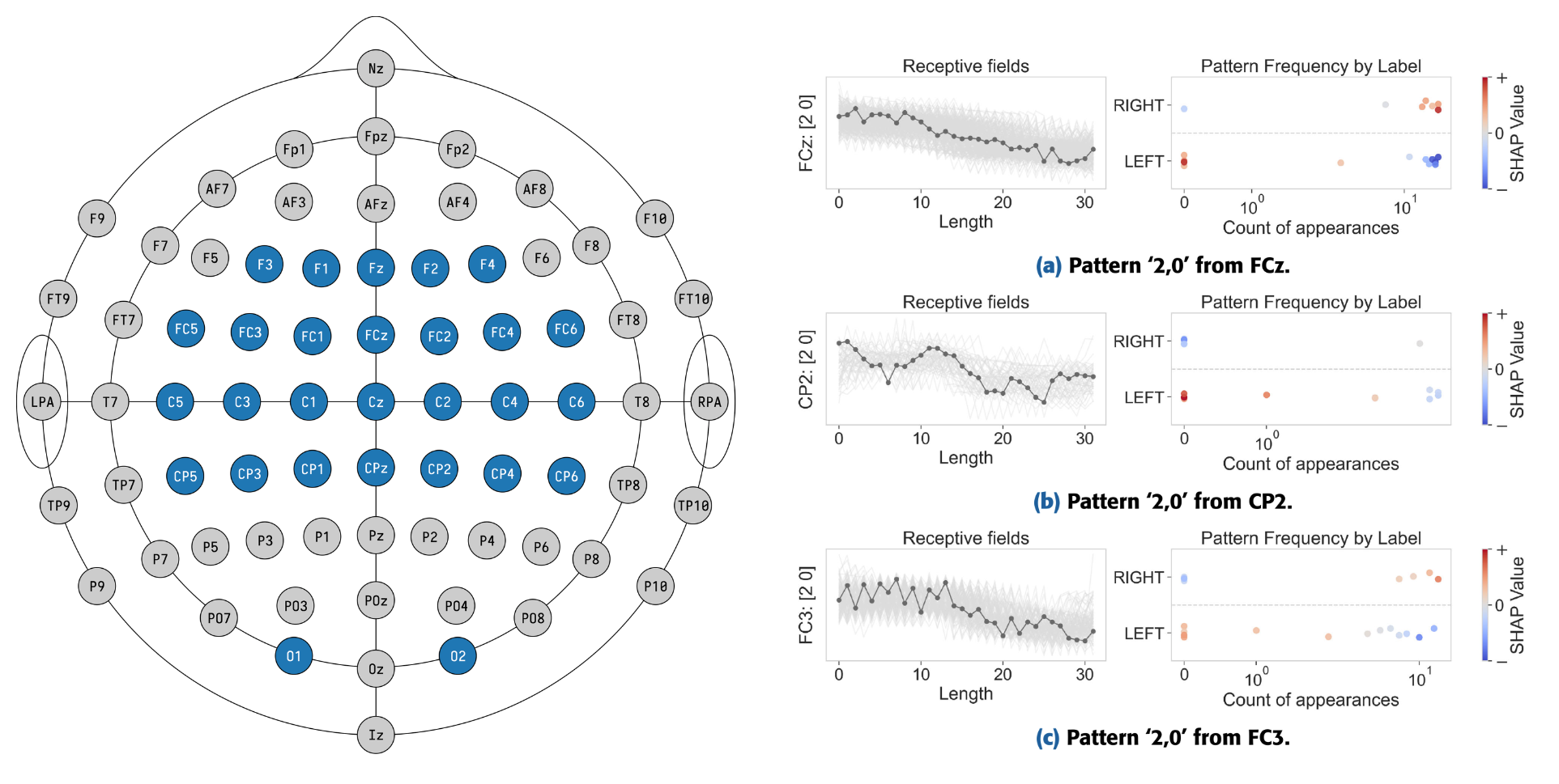
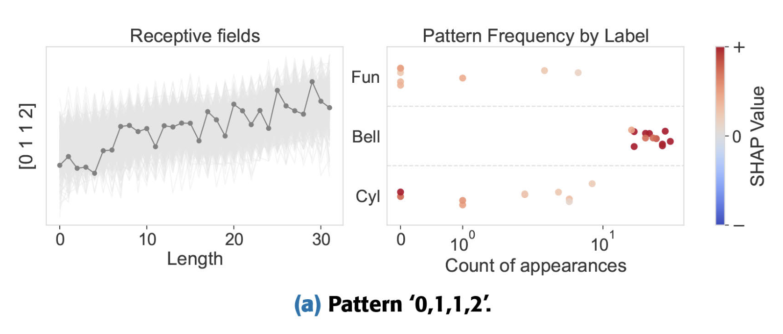
The global explanation below shows the behavior of the pattern in the full dataset. On the left, the medoid (in dark gray), and all possible alignments of that pattern in the dataset (light gray). On the right, we show the frequency of that pattern (x-axis) depending on the label (y-axis), colored by its importance. So low-medium-medium-high is contained many times in Bell instances, and when that pattern is contained many times, it pushes the prediction towards Bell. When the pattern is contained only a few times, or not contained at all, it pushes the prediction either towards Cylinder or Funnel.

We also test the approach on real-world datasets like FingerMovements. Here is the paper reference for more details:

@article{spinnato2024fast,
  title={Fast, interpretable and deterministic time series classification with a bag-of-receptive-fields},
  author={Spinnato, Francesco and Guidotti, Riccardo and Monreale, Anna and Nanni, Mirco},
  journal={IEEE Access},
  year={2024},
  publisher={IEEE}
}